Tabulate hexadecimal colours from RGB image bands in R

This (mostly useless) nugget came out of a sophisticated and ridiculous side-project that a colleague initiated. We needed a tool that would pull a table of hexadecimal colours out of an image (you know, those weird # colours that R and HTML use?). We wanted to know the most common colours in a given image and couldn’t find a pre-built tool that did this. So I made one. Again, probably useless to anyone else, but here it is because, well, the ether isn’t saturated (yet).

The function actually pulls all the images (.jpg files) out of a given directory path and batch processes them, producing a unique output for each. The last piece of code combines the tables for multiple images and outputs a single coloured barplot.

For this example, I have used two images from the iconic 1996 film ‘Pulp Fiction’, both of which are certainly subject to all kinds of copyright that should prevent me from posting them, but whatever. Download them and put them in a directory (within your working directory) called “Pulp Fiction”.

And here’s the code:

# Required packages
library('raster')
library('jpeg')
library('colorspace')
library('plyr')

# Directory title (must be in the working directory)
name <- "Pulp Fiction"

# Path to images (also the output path for tables & images)
filepath <- paste(name,"/",sep="")

# List of image files (will be used to name outputs)
image.list <- list.files(filepath,pattern=".jpg")
image.list <- substr(image.list,1,nchar(image.list)-4)

## FUNCTION ##
make.rgb.fun <- function(jpeg, round.dig, n.col){
 # Image must have a .jpg extension (NOT .jpeg)
 # jpeg = file name of image (without the .jpg extension)
 # round.dig = number of digits to round RGB values to (more = more unique but similar colours)
 # n.col = number of unique colour to plot 
 
 # Import image
 img <- readJPEG(paste(filepath,jpeg,".jpg",sep=""))
 
 # Extract RGB layers
 # Note the rounding of the RGB values
 img.R <- round(img[,,1],1) # RED
 img.G <- round(img[,,2],1) # GREEN
 img.B <- round(img[,,3],1) # BLUE
 
 # Make unique colours
 rgb <- hex(RGB(c(img.R),c(img.G),c(img.B)))
 rgb.tab <- as.data.frame(table(rgb))
 rgb.tab <- rgb.tab[order(-rgb.tab[2]),]
 rgb.tab$Prop <- round(rgb.tab$Freq/sum(rgb.tab$Freq),5)
 rgb.tab[1:10,]; dim(rgb.tab)
 cols <- as.character(rgb.tab[1:n.col,1])
 
 # Save hex colour table
 write.csv(rgb.tab, paste(filepath,jpeg,"_RGB_Table.csv",sep=""), row.names=F)
 
 # Plot
 graphics.off(); x11(w=12,h=5)
 layout.show(6)
 par(mfrow=c(2,4), mar=c(1,1,1,1))
 image(t(img.R[nrow(img.R):1L,]),axes=F, col=colorRampPalette(c("white","red"))(10))
 image(t(img.G[nrow(img.G):1L,]),axes=F, col=colorRampPalette(c("white","green"))(10))
 image(t(img.B[nrow(img.B):1L,]),axes=F, col=colorRampPalette(c("white","blue"))(10))
 plot(1:100,1:100,type="n",axes=F,ann=F); rasterImage(img,1,1,100,100)
 par(mar=c(5,5,1,1))
 hist(img.R, breaks=12, col="pink", xlab="RED", ylab="", las=1, main="")
 hist(img.G, breaks=12, col="darkolivegreen1", xlab="GREEN", ylab="", las=1, main="")
 hist(img.B, breaks=12, col="lightblue", xlab="BLUE", ylab="", las=1, main="")
 par(mar=c(8,1,1,1))
 barplot(rep(n.col,n.col), col=cols, axes=F, names.arg=cols, las=2)
 savePlot(paste(filepath,jpeg,"_RGB.png",sep=""),type="png")
}

# Run the function for the image list
# Rounds to 1 decimal, 15 colour output
lapply(image.list, make.rgb.fun, 1, 15)

For each of the images, you should have an output like this…

 

…as well as a .csv table with the complete list of unique colours, including the number and proportion of pixels in the image of that colour.

   rgb     Freq   Prop
1  #000000 236295 0.30046
2  #DA5900 90143  0.11462
3  #DA5959 40361  0.05132
4  #595900 32629  0.04149
... 

Here is where you’ll notice the effect of rounding the RGB values. If you leave them more precise (i.e. more decimals), you’ll end up with many more unique colours and many nearly identical colours repeated in the image. Do what you like.

With multiple images, the last piece of code creates a combined colour plot (using the proportions, so you need not worry about combining low and high resolution images).

# Combine all the images
rm(dat)
for(i in image.list){
 if(i==image.list[1]){
 dat <- read.csv(paste(filepath,i,"_RGB_Table.csv",sep=""))
 } else {
 dat <- rbind(dat,read.csv(paste(filepath,i,"_RGB_Table.csv",sep="")))
 } 
}
# Combine duplicate values
dat <- ddply(dat, .(rgb), summarise, Prop=round(sum(Prop)/length(image.list),5))
dat <- dat[order(-dat$Prop),]
head(dat); dim(dat)
# Save the table
write.csv(dat, paste(filepath,name,"_Combined_Hex_Table.csv",sep=""), row.names=F)
# Plot combined colours
graphics.off(); x11()
par(mar=c(1,6,2,2))
n.cols <- 30
barplot(rep(n.cols,n.cols), axes=F, col=rev(as.character(dat[1:n.cols,"rgb"])), names.arg=rev(as.character(dat[1:n.cols,"rgb"])), las=2, main=name, horiz=T)
# Save the plot
savePlot(paste(filepath,name,"_Combined_Hex_Plot.png",sep=""),type="png")

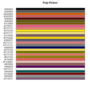
The output plot will look something like this:

Now, you can pull your favourite colours off the plot (with the handy # hex code printed in the margin). Have fun at home with your friends making colour palettes for your favourite internet images! Woohoo!

WEAK CREDIT: the included function uses a .jpg plotting code that I found on StackExchange. I would credit it to the thread, but can’t now seem to relocate it. Sorry to the person who posted it. I hope karma finds you (and not me).